Model Drift and Monitoring

Overview

Choose this use case if you want to monitor a deployed model in production.

To follow this tutorial, ensure you have followed these steps:

1. Log in to the Abacus developer platform
2. Create a new project of type "Model Drift and Monitoring"
3. Provide a name, and click on Skip to Project Dashboard.

If you are having trouble creating a new project, follow this guide

Note: When training a Machine Learning model in Abacus using our built-in project types, you can monitor deployments directly from your project dashboard. However, this use case is specifically designed for scenarios where you're working with models built outside Abacus—allowing you to leverage Abacus exclusively as a model monitoring system by ingesting external training data and predictions.

Steps to Create a Custom Monitor

Step 1: Ingest data into the platform

Once you are ready to upload data, follow these steps:

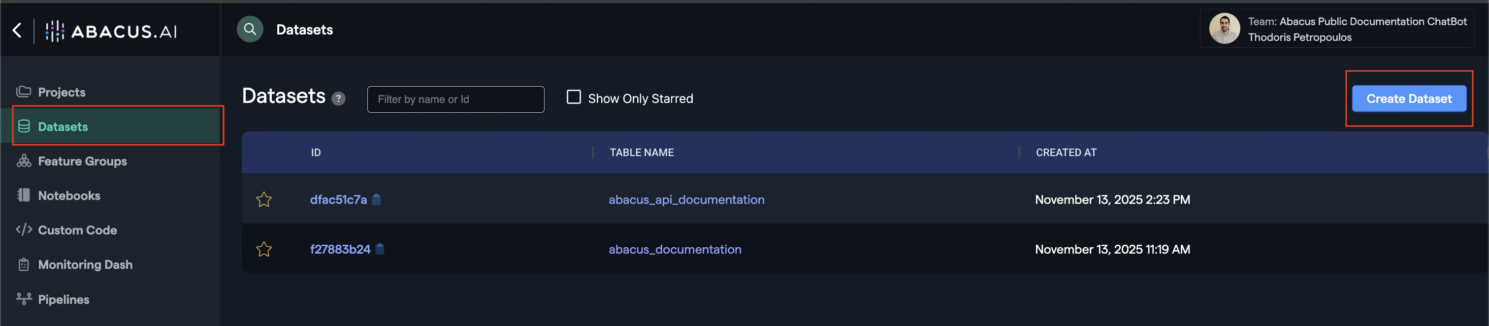
1. Click on Datasets within the project page on the left side panel.
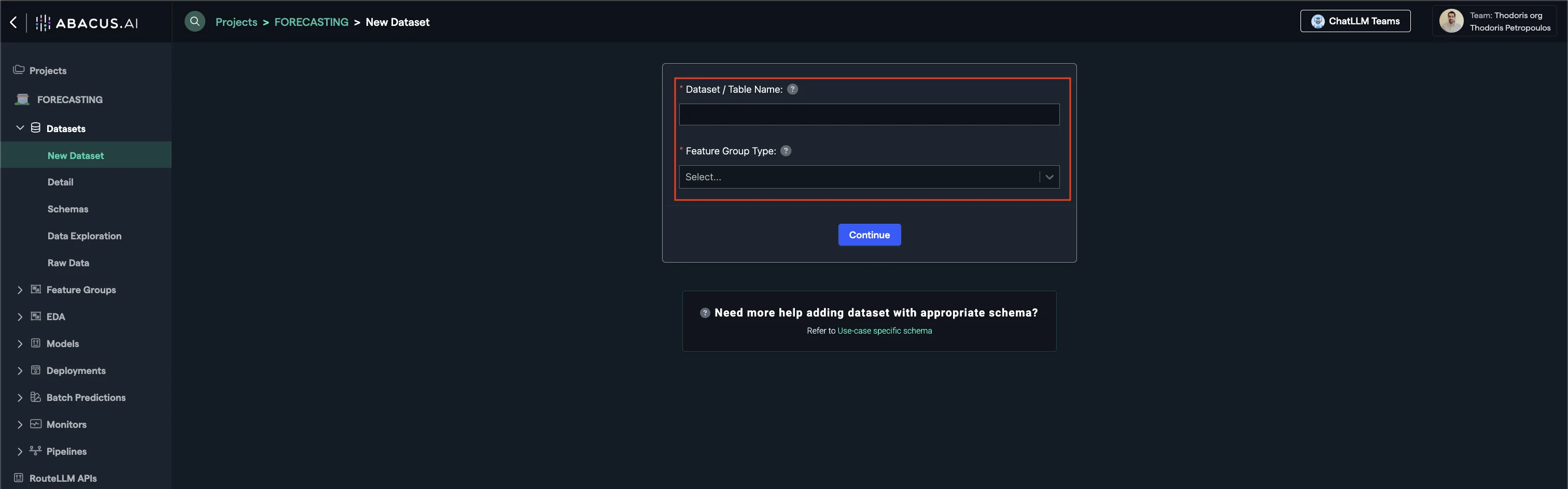
2. Click on Create Dataset on the top right corner.
3. IMPORTANT: Provide a name and upload one of each:
   • TRAINING_DATA feature group type
   • PREDICTION_LOG feature group type

Step 2: Configuring Feature Groups

Once the dataset has finished inspecting, navigate to the Feature Group area from the left panel. You should be able to see a Feature Group that has the same name as the dataset name you provided.

1. Navigate to Feature group → Features
2. Select the appropriate feature group type (see Required Feature Groups)

To learn more about how feature group mapping works, visit our Feature Group mapping guide for detailed configuration instructions.

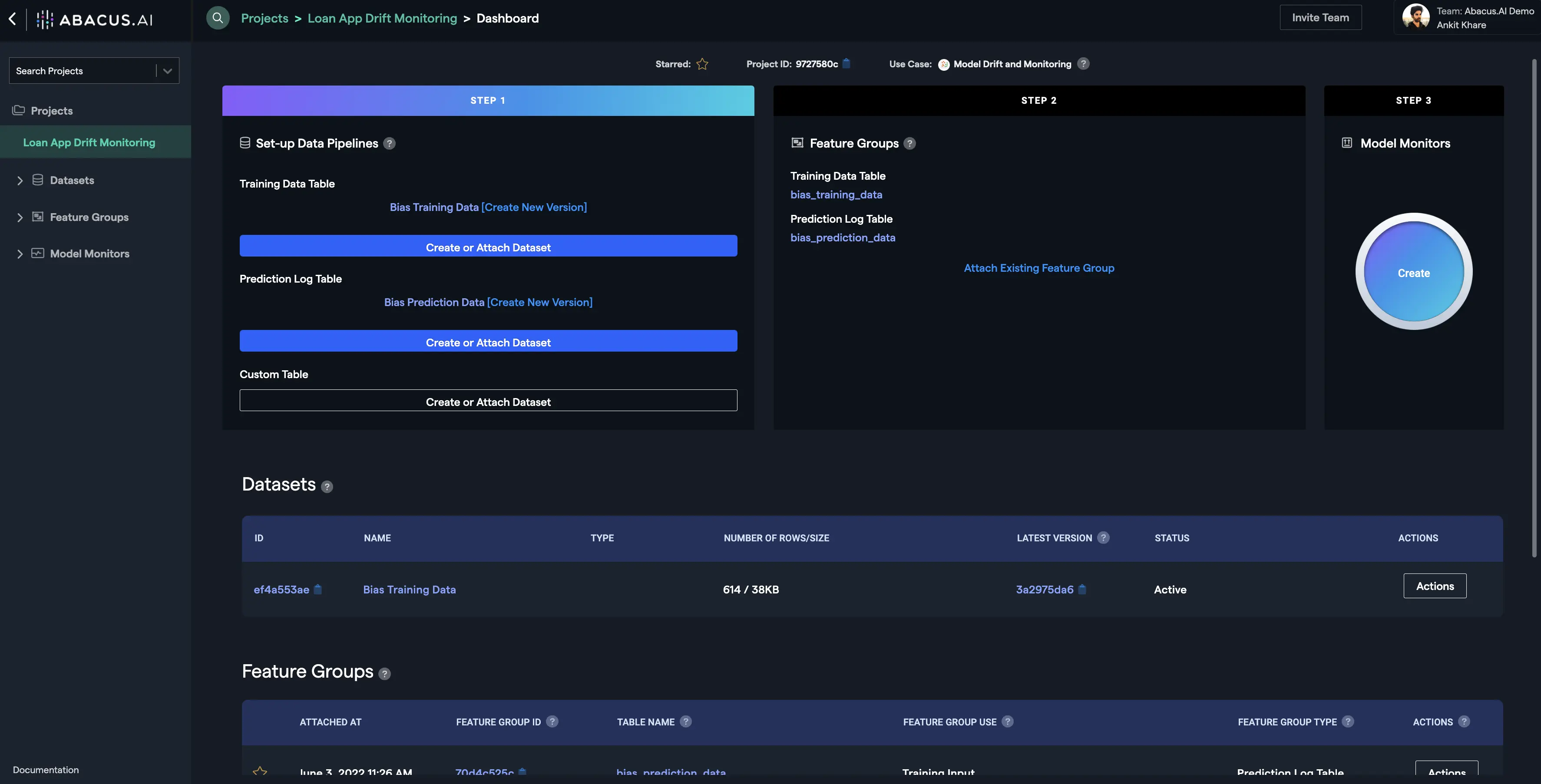
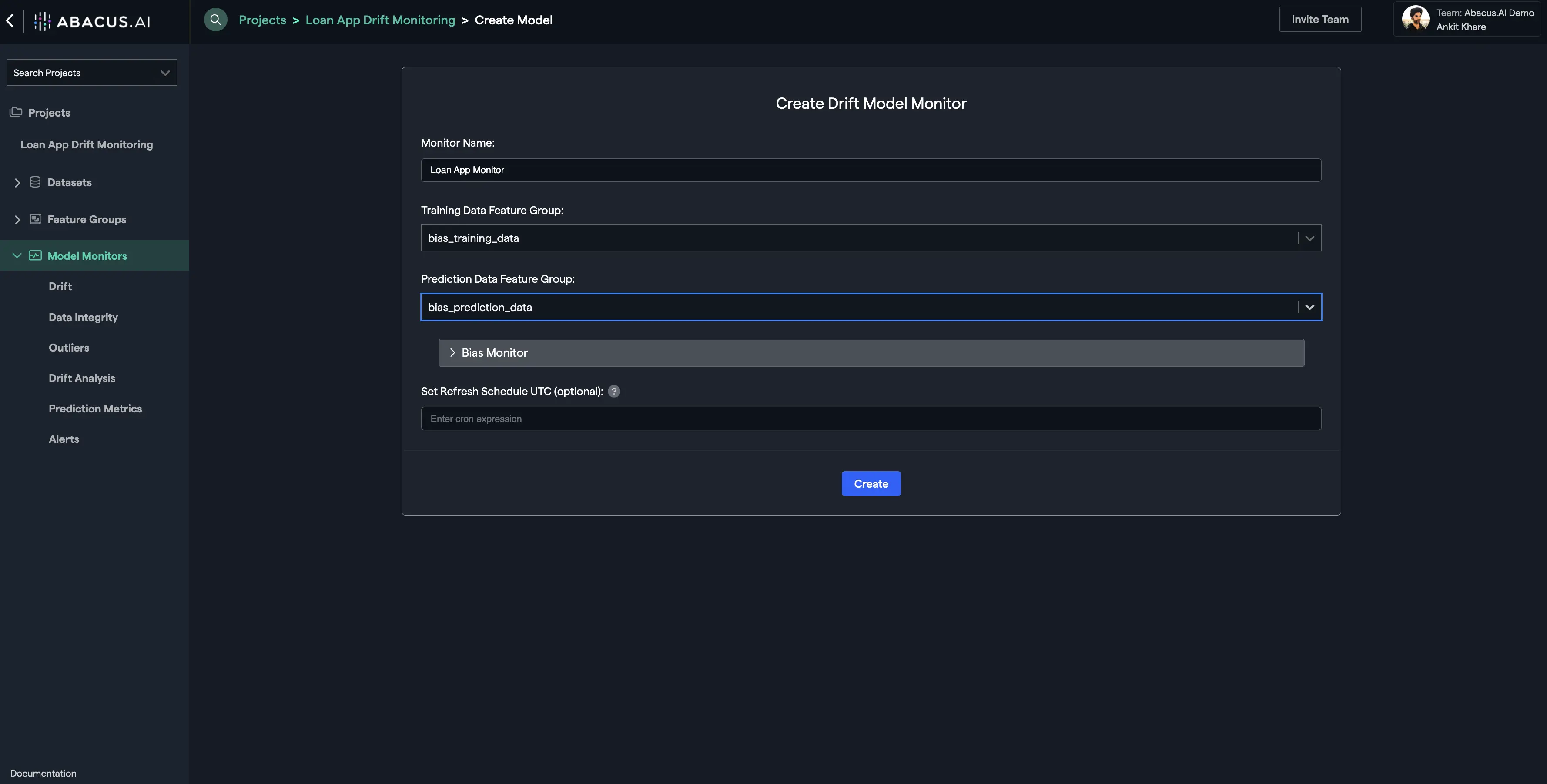
Step 3: Creating a monitor

Once you fulfill the Feature Group Type requirements and the feature mapping requirements, you are ready to create a Model Monitor. Click on the "Create" button under Step 3 on the project dashboard, select the training and prediction feature groups, and finally click on the "Create" button:

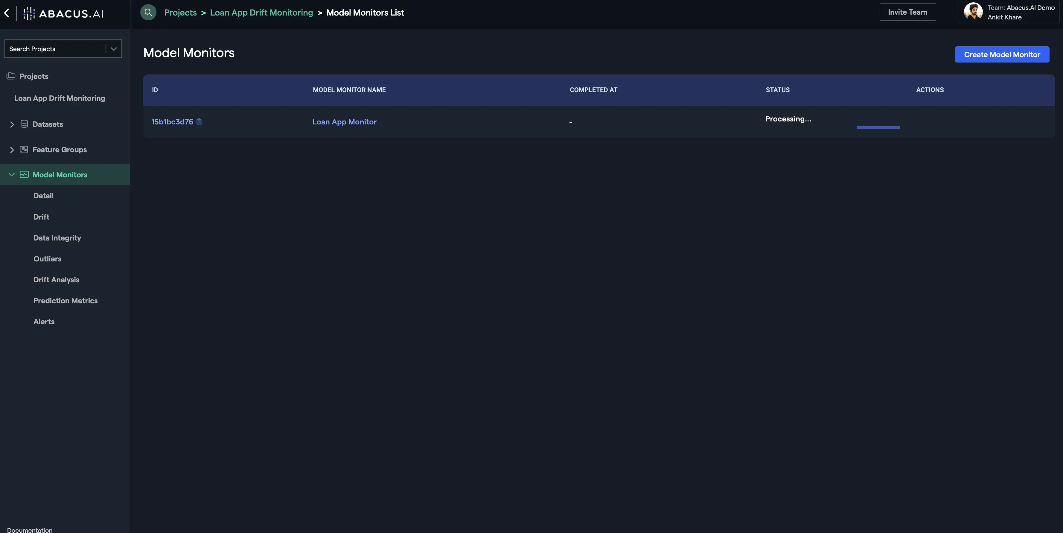
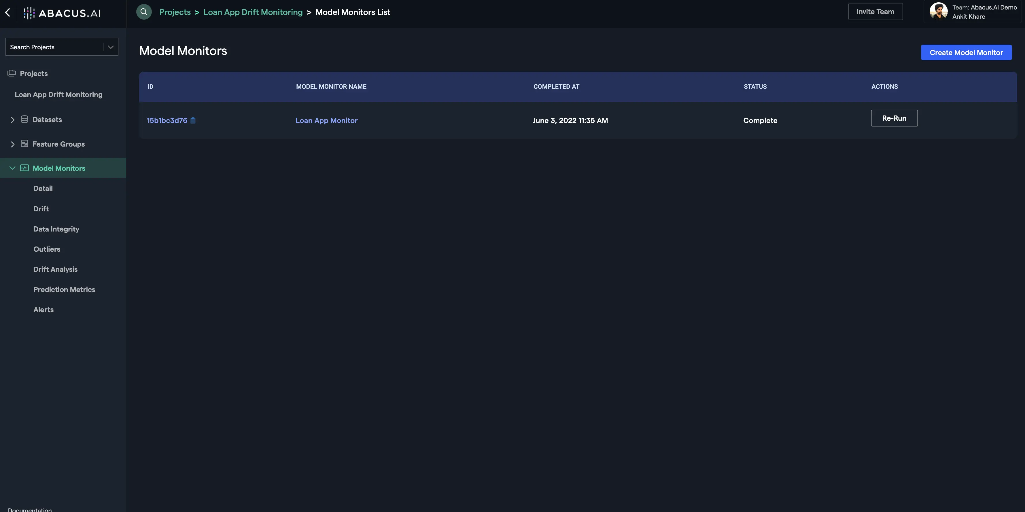
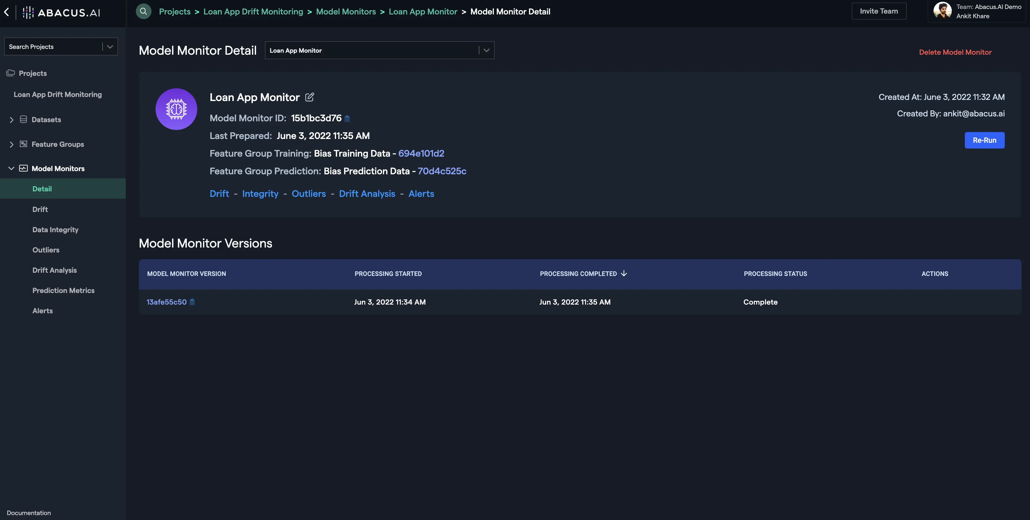
Once the processing finishes, you will see be able to see the model monitor details and utilize all the functionalities under the option "Model Monitors" at the left navigation:

Drift

Drift is calculated for the target variable as Prediction Drift and as Feature Drift for the features that were used to train the model.

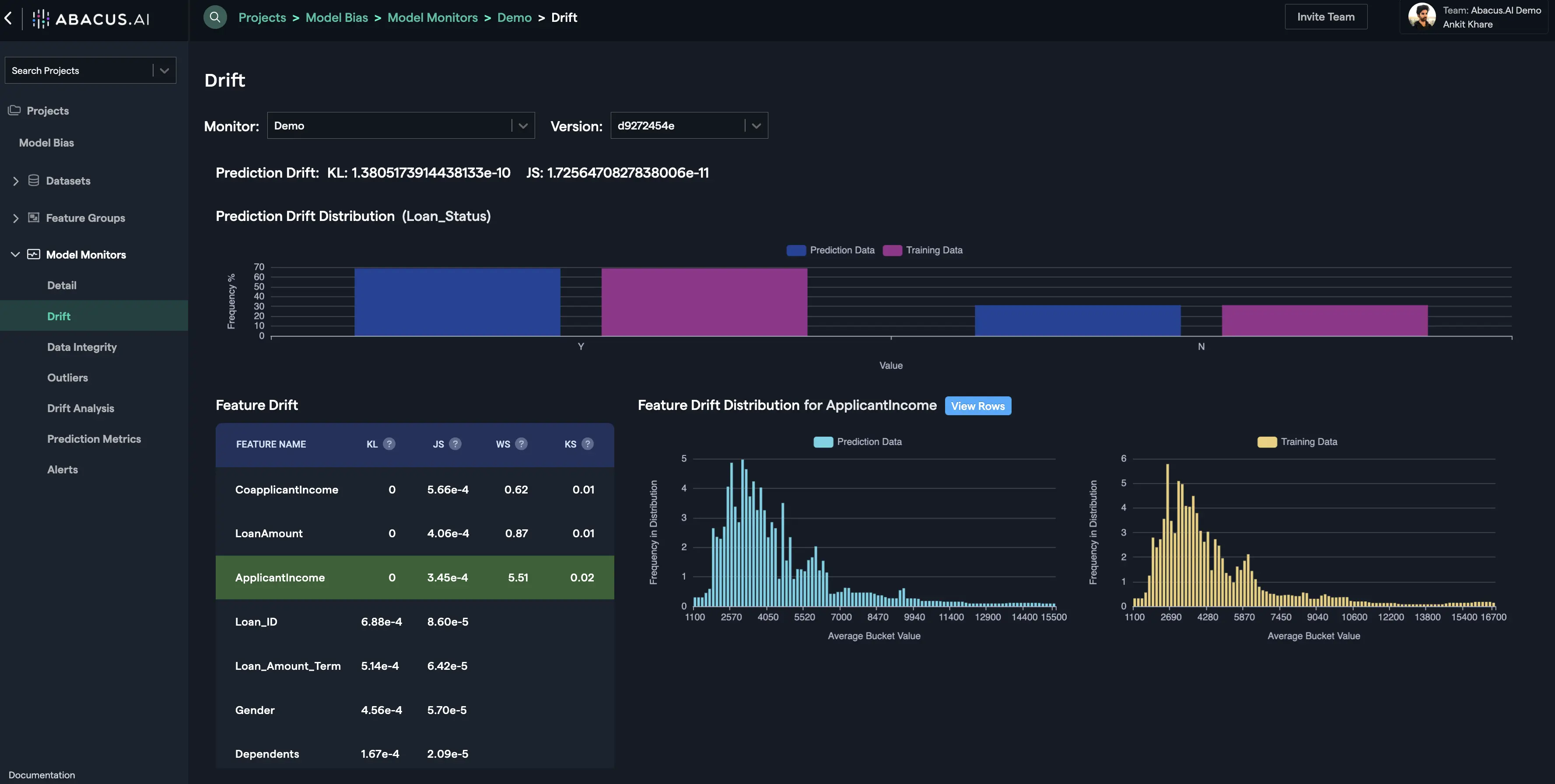
Prediction Drift

Prediction Drift is calculated using the differences in the distribution of the target variable. For e.g., let's suppose that the target variable is loan_status that shows if the loan was granted or not, then the frequency (in percentage) of the value 'Y' and 'N' for the prediction data and the training data are displayed as Prediction Drift Distribution. KL divergence and JS distance are calculated using the training and the prediction data for the target variable and shown as Prediction Drift.

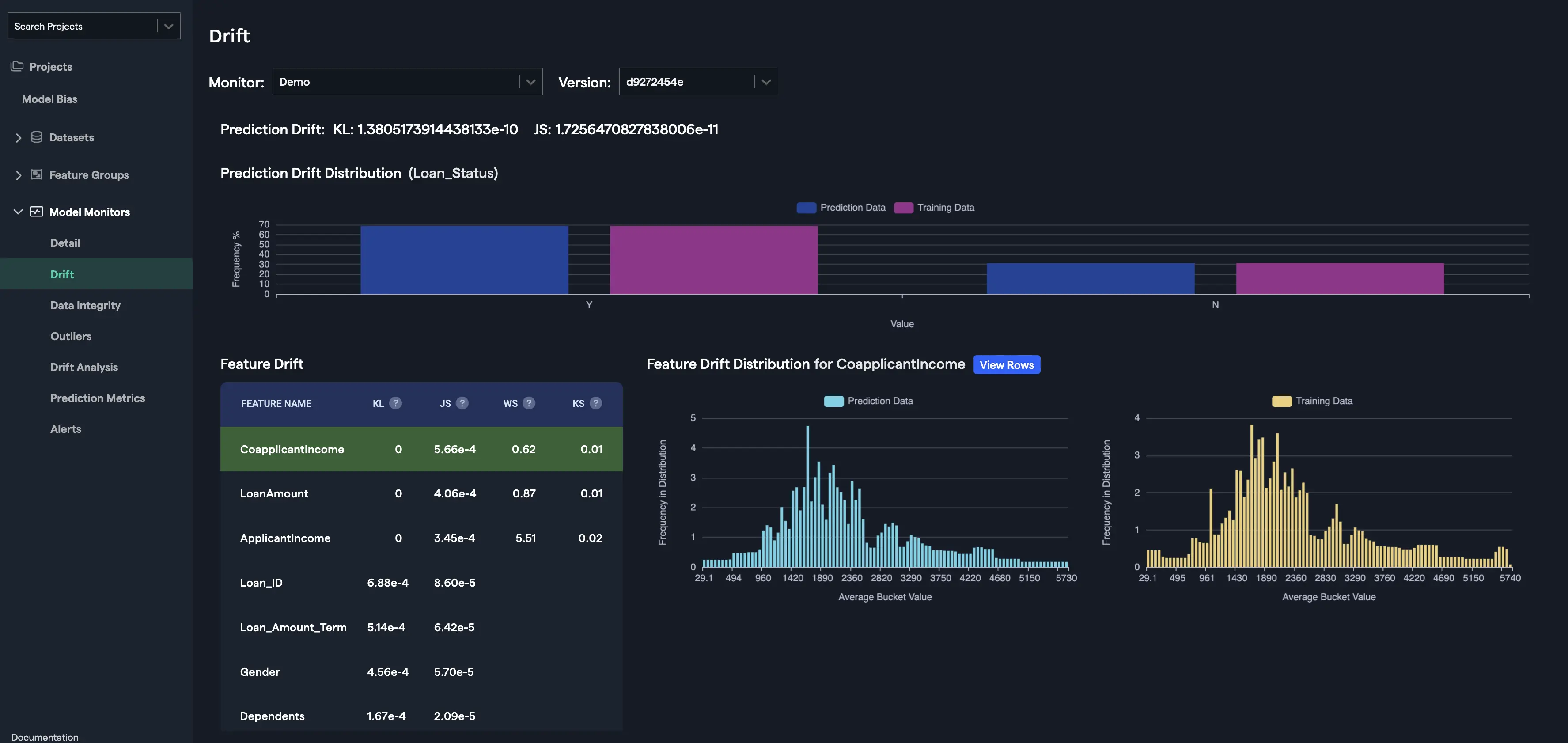
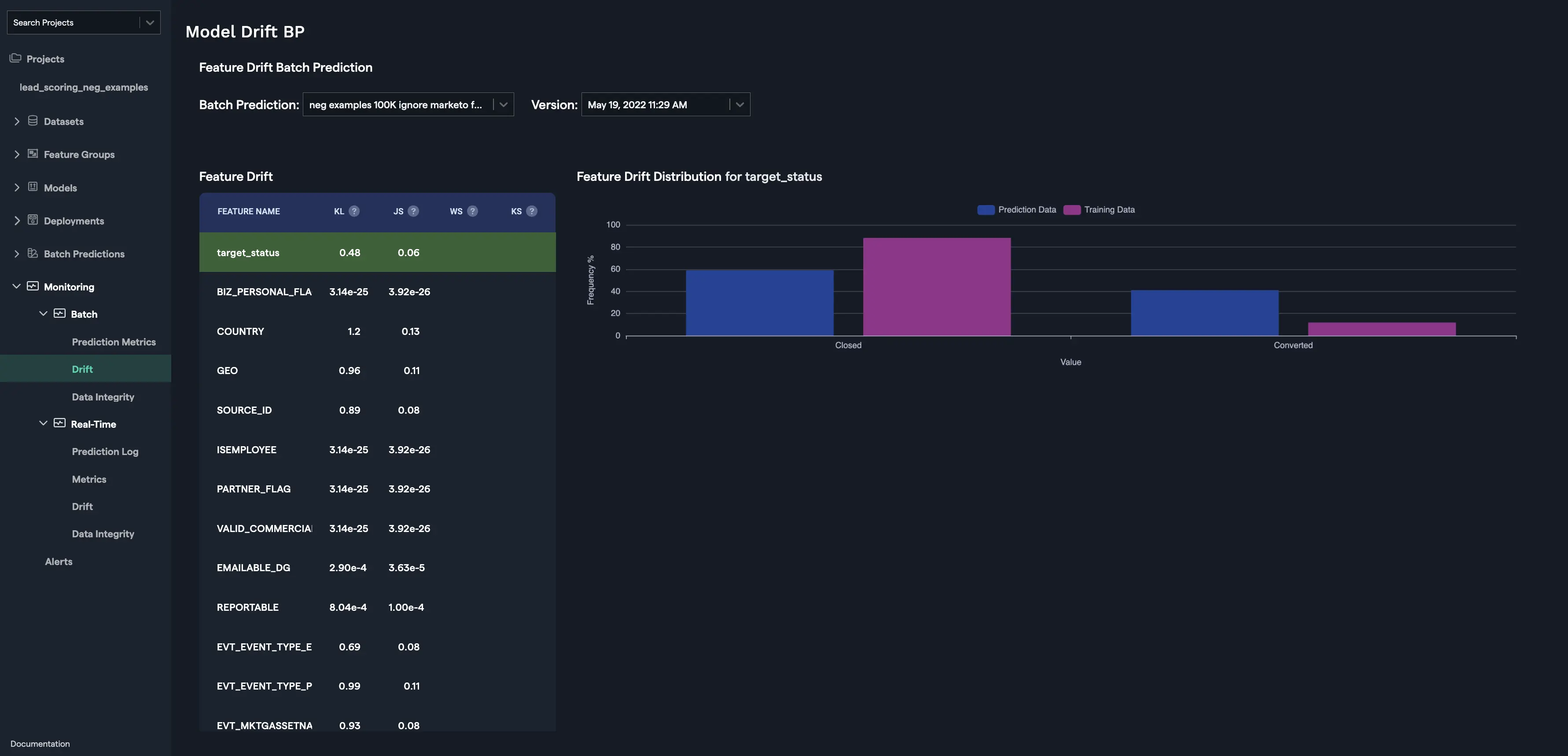
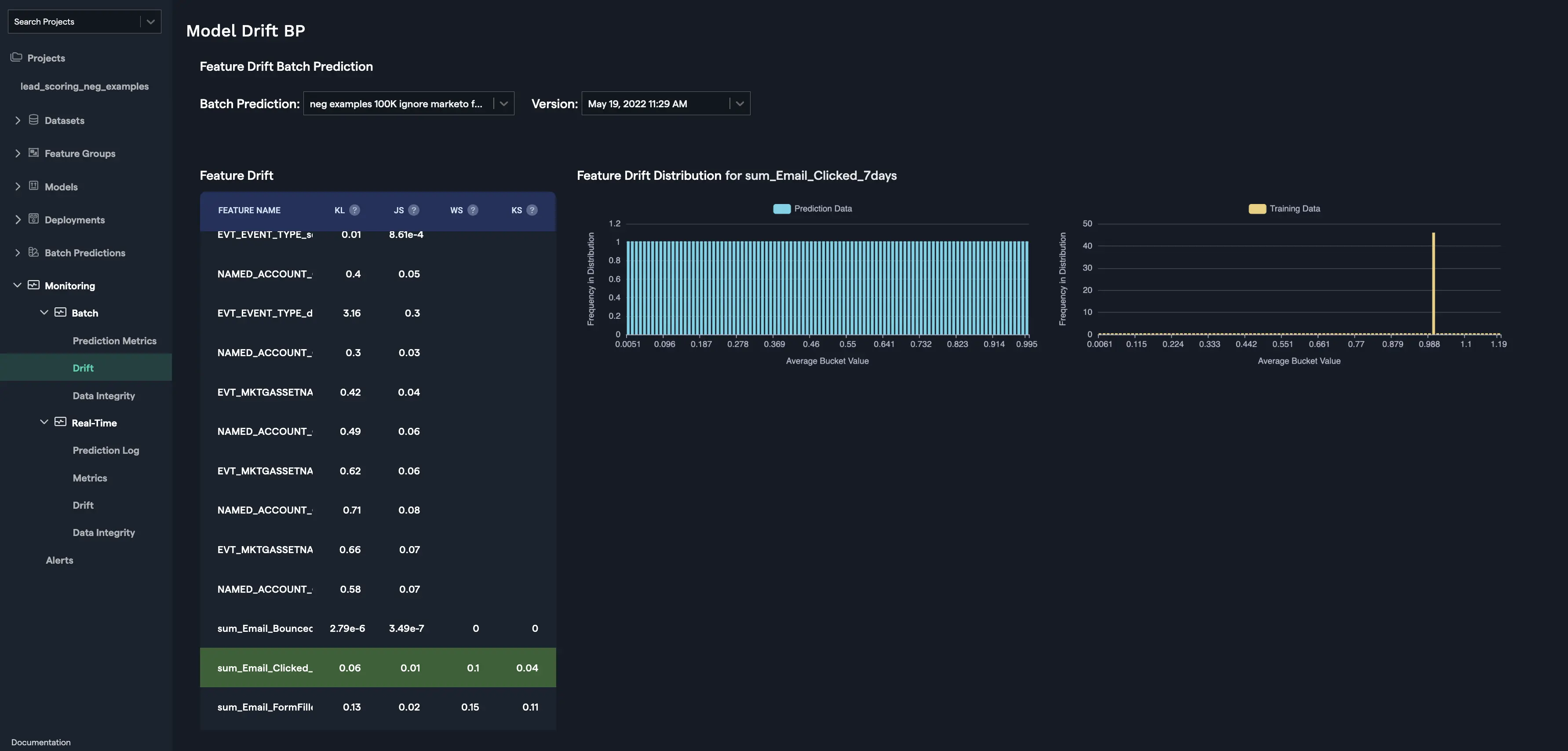
Feature Drift

Feature Drift is calculated for each feature using the differences in the distribution of the feature. Four types of distances calculated to estimate feature drift depending upon the type of the feature (categorical, numerical, etc.) are as follows:

KL Divergence

The Kullback-Leibler Divergence score, or KL divergence score, quantifies how much one probability distribution differs from another probability distribution. The intuition for the KL divergence score is that when the probability for an event from P is large, but the probability for the same event in Q is small, there is a large divergence. When the probability from P is small and the probability from Q is large, there is also a large divergence, but not as large as the first case.

It can be used to measure the divergence between discrete and continuous probability distributions, where in the latter case the integral of the events is calculated instead of the sum of the probabilities of the discrete events. For more details, visit this page.

JS Distance

The Jensen-Shannon distance measures the difference between two probability distributions. For example, suppose P = [0.36, 0.48, 0.16] and Q = [0.30, 0.50, 0.20]. The Jenson-Shannon distance between the two probability distributions is 0.0508. If two distributions are the same, the Jensen-Shannon distance between them is 0.

Jensen-Shannon distance is based on the Kullback-Leibler divergence. In words, to compute Jensen-Shannon between P and Q, you first compute M as the average of P and Q and then Jensen-Shannon is the square root of the average of KL(P,M) and KL(Q,M). In symbols:

JS(P,Q) = sqrt( [KL(P,M) + KL(Q,M)] / 2 ) where M = (P + Q) / 2

For more details, visit this page.

Wasserstein Distance

Imagine the two datasets to be piles of earth, and the goal is to move the first pile around to match the second. The Earth Mover's Distance is the minimum amount of work involved, where "amount of work" is the amount of earth you have to move multiplied by the distance you have to move it. The EMD can also be shown to be equal to the area between the two empirical CDFs. As the EMD is unbounded, it can be harder to work with, unlike for the KS distance which is always between 0 and 1. For more details, visit this page.

KS Distance

The first distance that we consider comes from the well-known Kolmogorov-Smirnov test (KS). To compare the two datasets, we construct their empirical cumulative distribution functions (CDF) by sorting each set and drawing a normalized step function that goes up at each data point. The KS distance is defined to be the largest absolute difference between the two empirical CDFs evaluated at any point.

In fact, we can call it a distance, or metric, because it satisfies four conditions that formalize the intuitive idea that we have of a distance:

• its value is greater than or equal to zero,
• it is equal to zero if and only if both distributions are identical,
• it is symmetric: the distance from one distribution to another is equal to the distance from the latter to the former,
• if A, B and C are distributions, then KS(B,C)≤KS(B,A)+KS(A,C), or intuitively, with the definition of KS, it is shorter to go straight from B to C rather than going through A, which is known as the triangle inequality.

Those properties make the KS distance powerful and convenient to use. The KS distance is always between 0 and 1, so it is of limited use when comparing distributions that are far apart. For example, if you take two normal distributions with the same standard deviation but different means, the KS distance between them does not grow proportionally to the distance between their means. This feature of the KS distance can be useful if you are mostly interested in how similar your datasets are, and once it's clear that they're different you care less about exactly how different they are. For more details, visit this page.

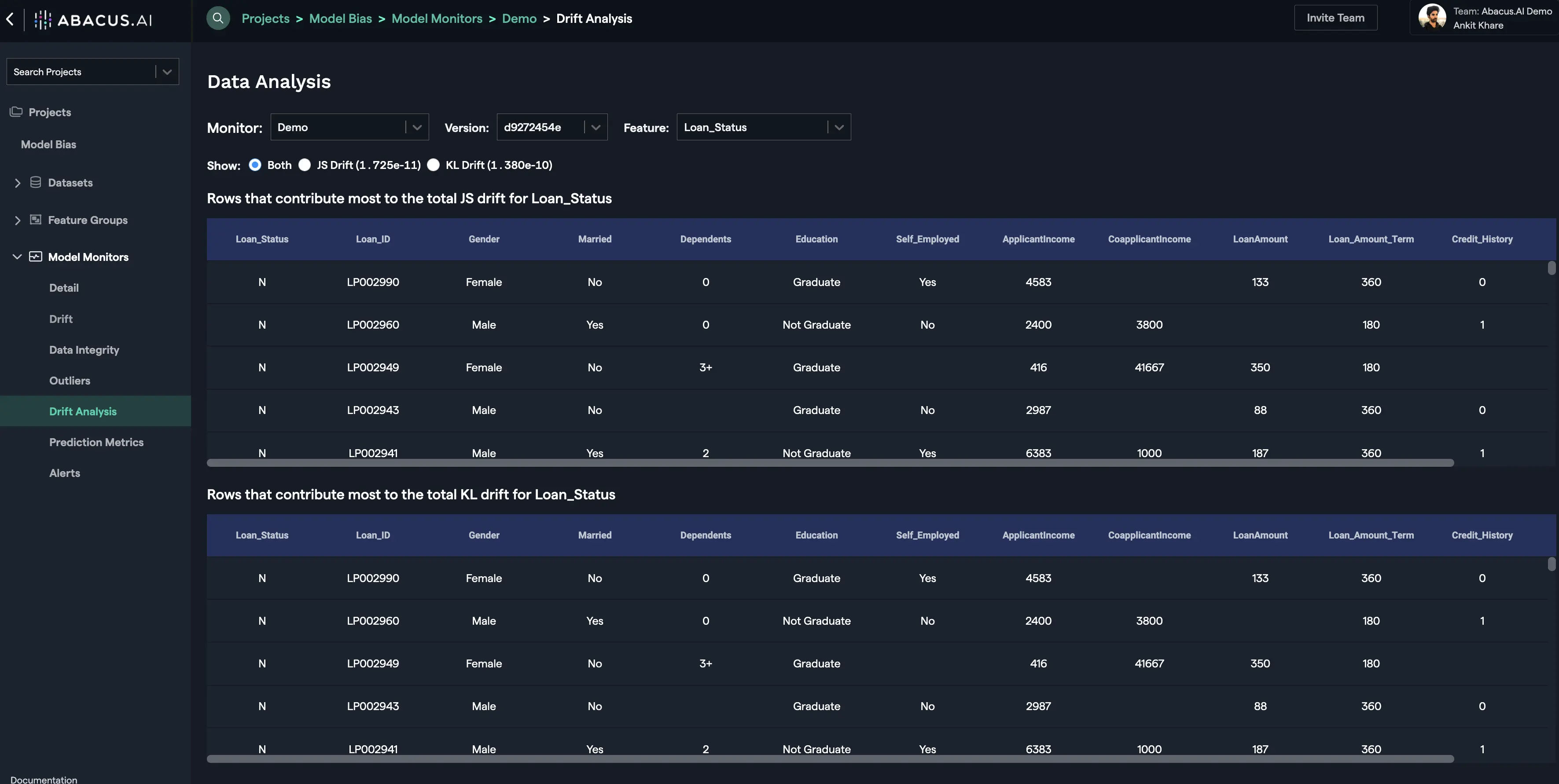
Drift Analysis

The rows / records that contribute most to the drift for the feature are displayed in the drift analysis interface. For each feature you will have the option to see the records that contribute the most for KL Drift and/or JS Drift. You can click on the "View Rows" button to go to the drift analysis interface for the particular feature or you can select the "Drift Analysis" option from the left navigation to see the drift analysis for any feature:

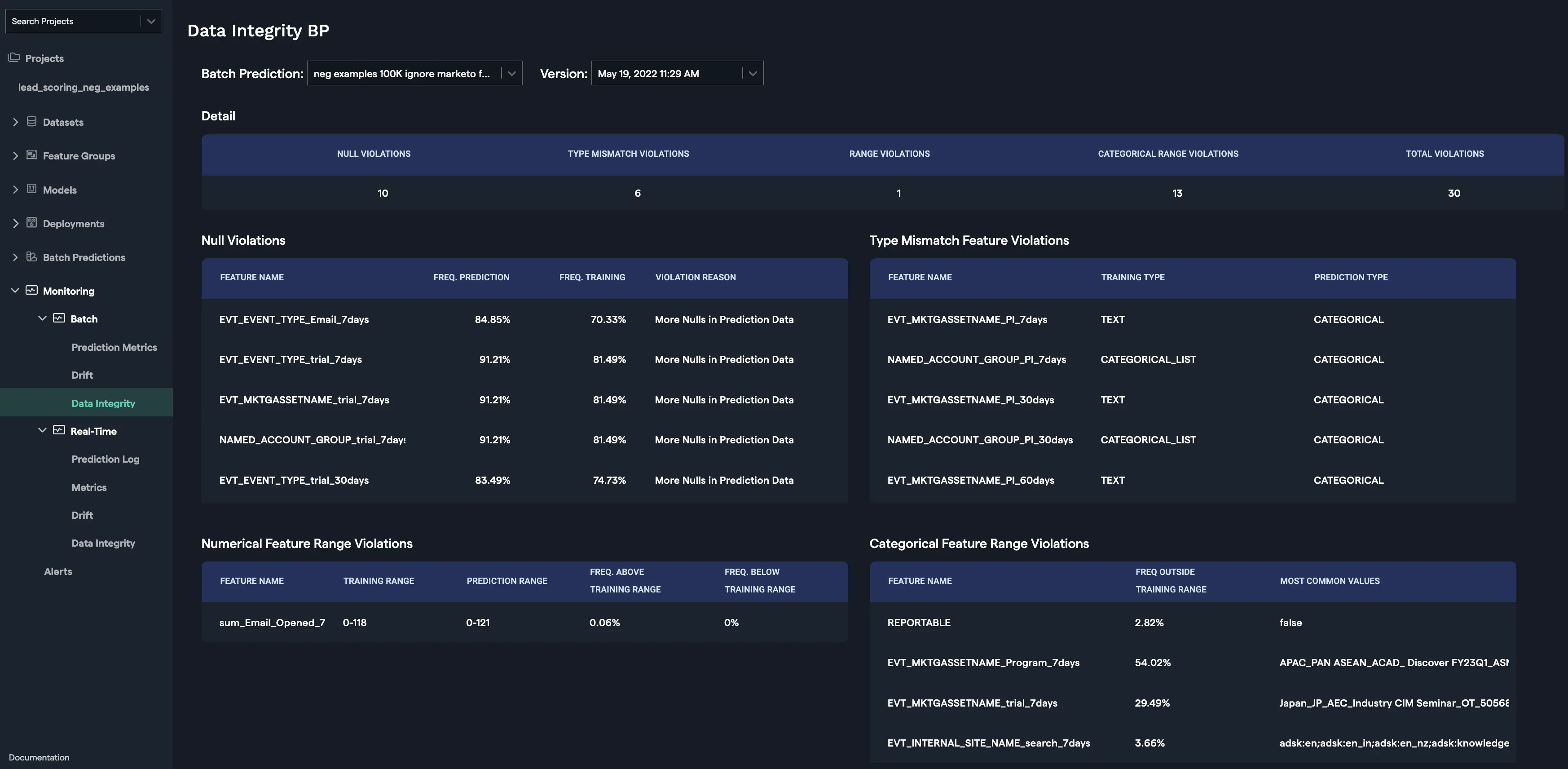
Data Integrity

The data integrity interface displays different kinds of mismatches between the training and prediction data. It is found under the "Monitoring" tab for both "Batch" and "Real-Time" sub-tabs. The interface remains the same for both "Batch" and "Real-Time" except that the real-time interface provides a Time Range (date range) to input a subset of the real-time data, whereas, the batch interface takes a specific batch prediction name and a version to display the associated mismatches. The four types of violations monitored are described as follows:

• Null violations - This occurs when a feature has an instance of a null value. Whenever there is a mismatch in the percentage of null violations within a feature between the training set and the prediction set, it is captured and displayed with a reason for the mismatch.

• Type mismatch violations - This occurs when a feature has mismatch in the feature type (categorical, numerical, etc.) between the training and the prediction data.

• Range violations - This occurs when a feature of type, "numerical", has a range mismatch between the training and the prediction data.

• Categorical Range Violations - This occurs when a feature of type, "categorical", has a range mismatch between the training and the prediction data.

  

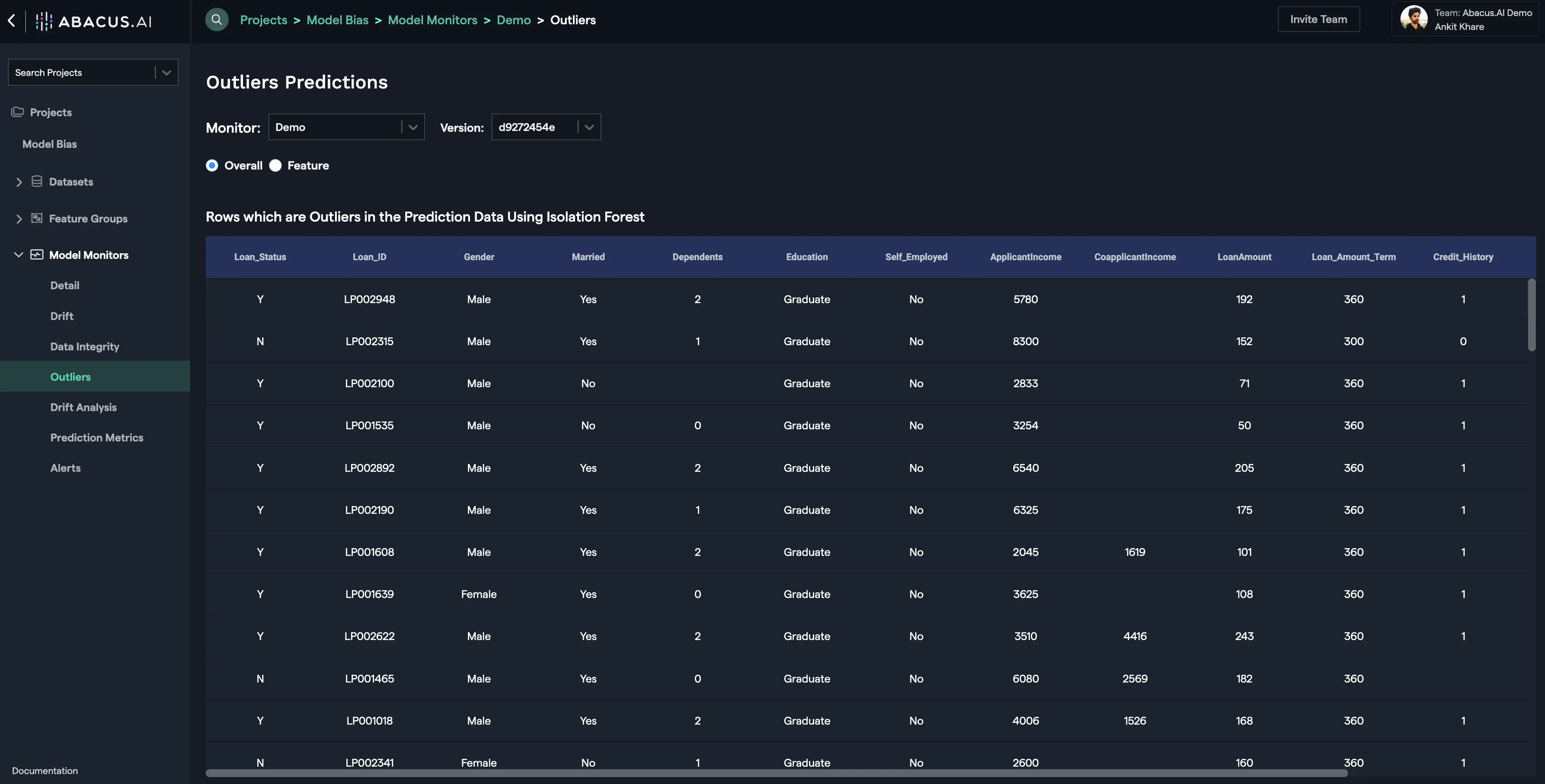
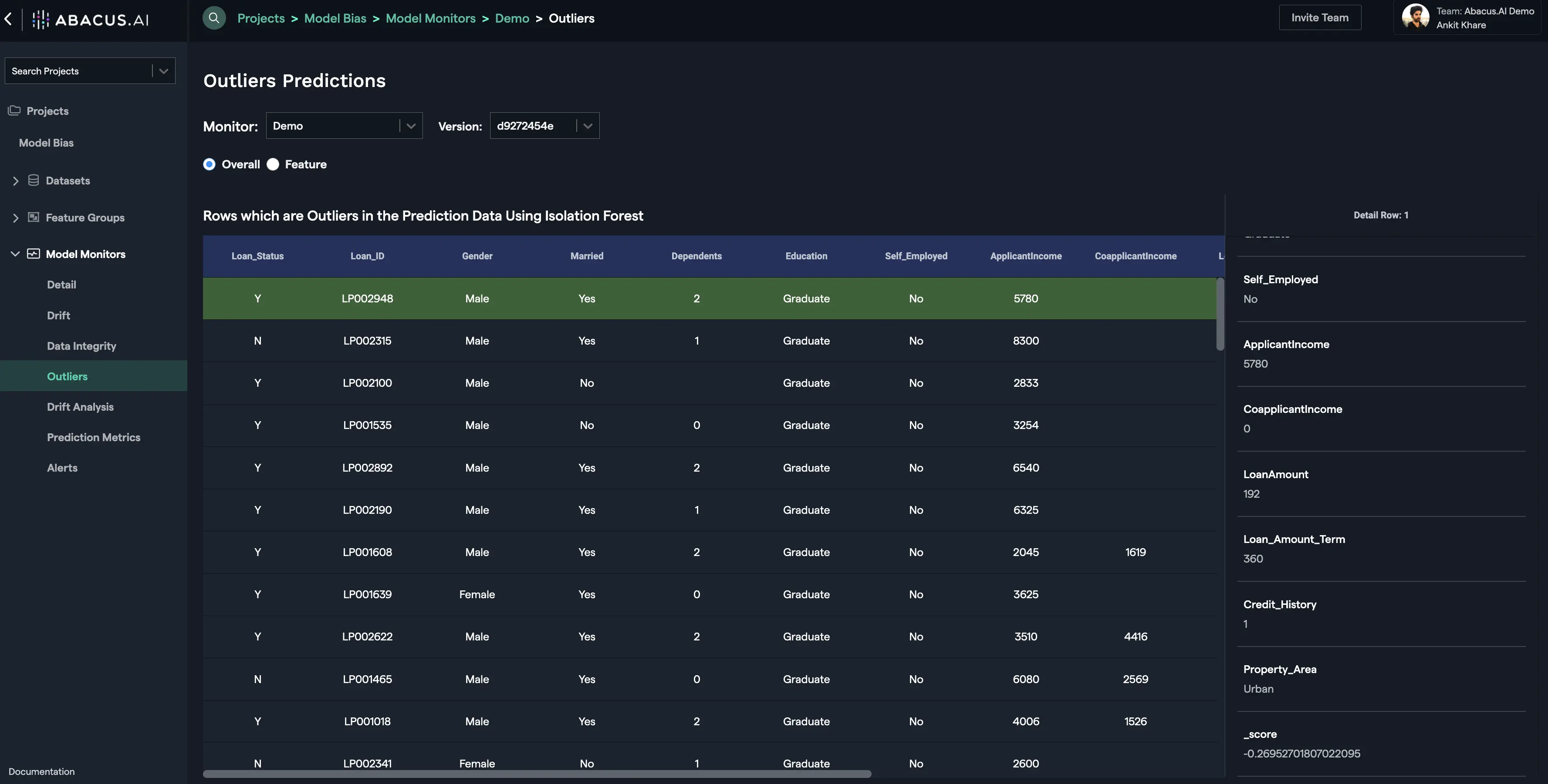
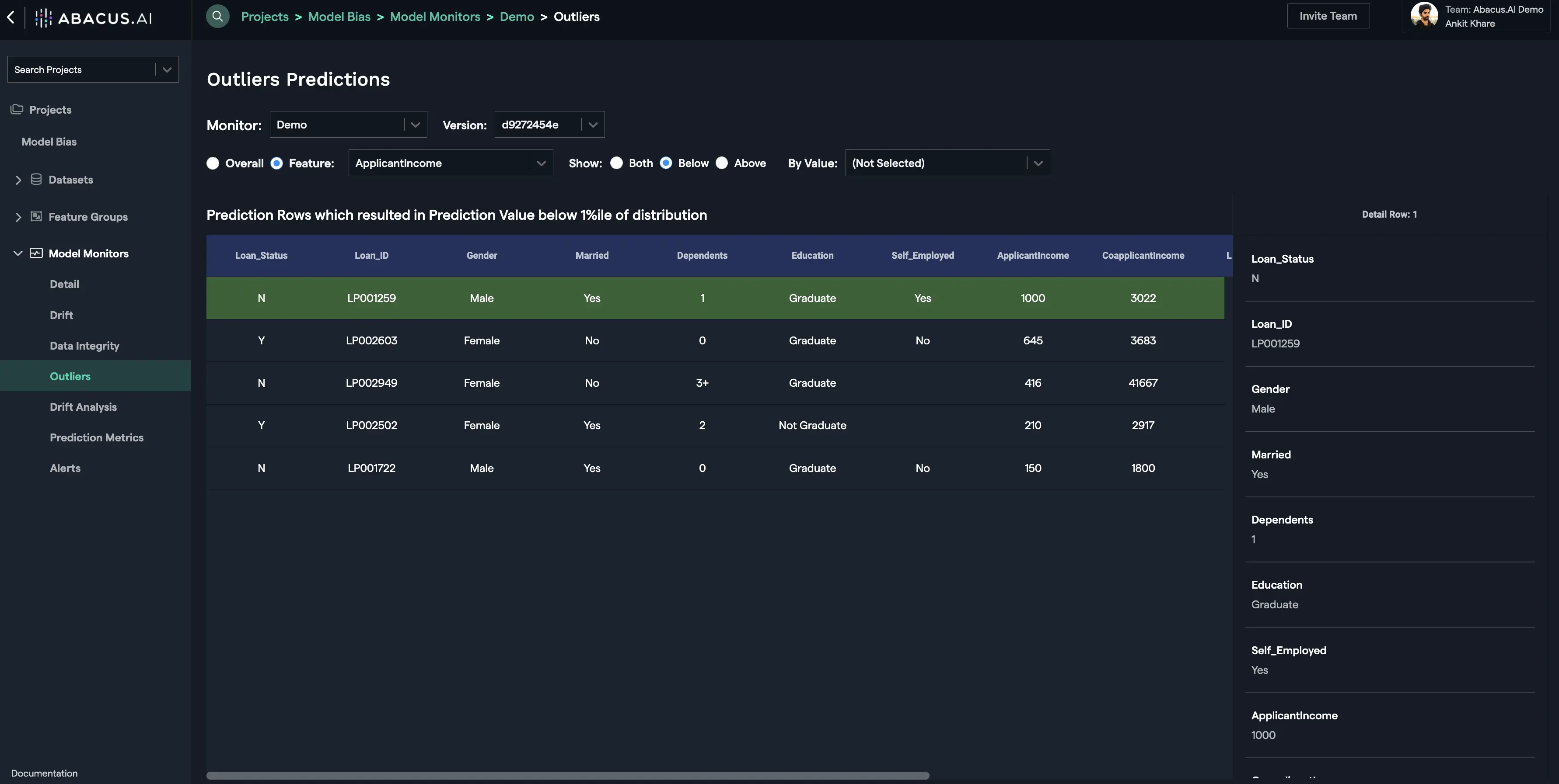
Outliers

This interface displays the outliers within the prediction data. There are two options available to monitor outliers: Overall and Feature. Overall option displays the anomalous rows (outliers) in the prediction data using the Isolation Forest method.

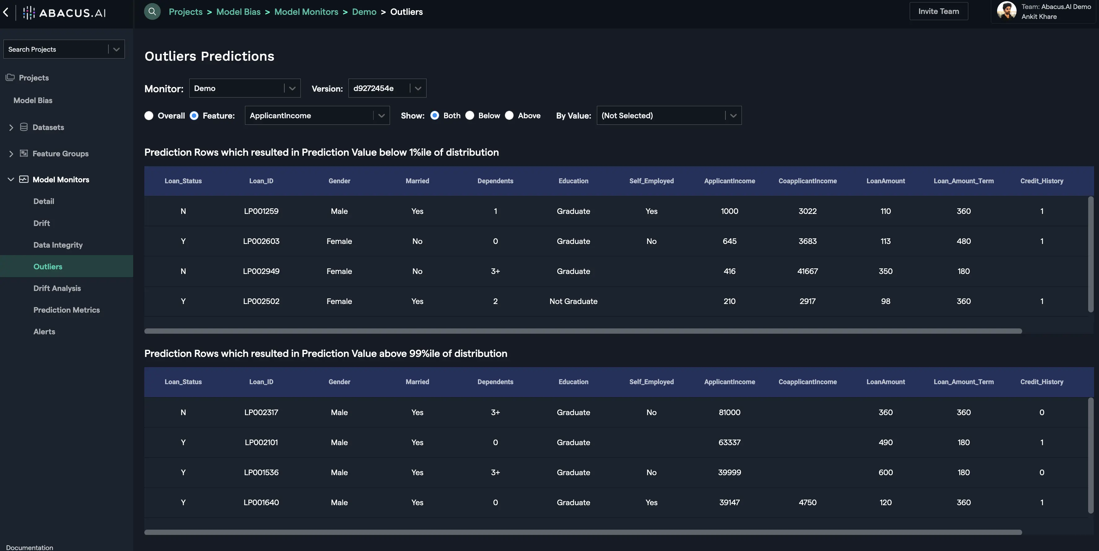
For the feature outliers, prediction rows that resulted in prediction value below 1 percentile of distribution and/or above 99 percentile of distribution are displayed:

Required Feature Group Types

Here are the types required to create a monitor:

Feature Group Type	API Configuration Name	Required	Description
Training Data Table	TRAINING_DATA	True	Dataset representing the distribution of features encountered by a model during training.
Prediction Log Table	PREDICTION_LOG	True	Dataset representing the distribution of features encountered by a model during prediction or deployment.

Note: Once you upload the datasets under each Feature Group Type that comply with their respective required schemas, you will need to create Machine learning (ML) features that would be used to train your ML model(s). We use the term, "Feature Group" for a group of ML features (dataset columns) under a specific Feature Group Type. Our system supports extensible schemas that enable you to provide any number of additional columns/features that you think are relevant to that Feature Group Type.

---

Feature Group: Training Data Table

Dataset representing the distribution of features encountered by a model during training.

Feature Mapping	Feature Type	Required	Description
TARGET		Y	The target value the model is training to predict
MODEL_VERSION	categorical	N	The unique identifier of the model version that was trained with this training row.
PREDICTED_VALUE		N	Model output value for this prediction data.
IMAGE	objectreference	N	Image reference
DOCUMENT		N	Document text

---

Feature Group: Prediction Log Table

Dataset representing the distribution of features encountered by a model during prediction or deployment.

Feature Mapping	Feature Type	Required	Description
PREDICTION_TIME	timestamp	N	Timestamp of the prediction.
ACTUAL		N	The ground truth value of this prediction data.
PREDICTED_VALUE		N	Model output value for this prediction data.
PREDICTED_PROBABILITY		N	Model output probability value for prediction data.
MODEL_VERSION	categorical	N	The unique identifier of the model version corresponding to the prediction.
PROTECTED_CLASS	categorical	N	Protected class to compute model bias metrics on.
IMAGE	objectreference	N	Image reference
DOCUMENT		N	Document text