Advanced Feature Generation: Nested Features and Point-In-Time Group
Learning Objectives
- Lag Features: How to create lag features automatically.
- Nested vs. Point-In-Time Features: Understanding the differences and use cases.
Watch the Tutorial
Add Feature
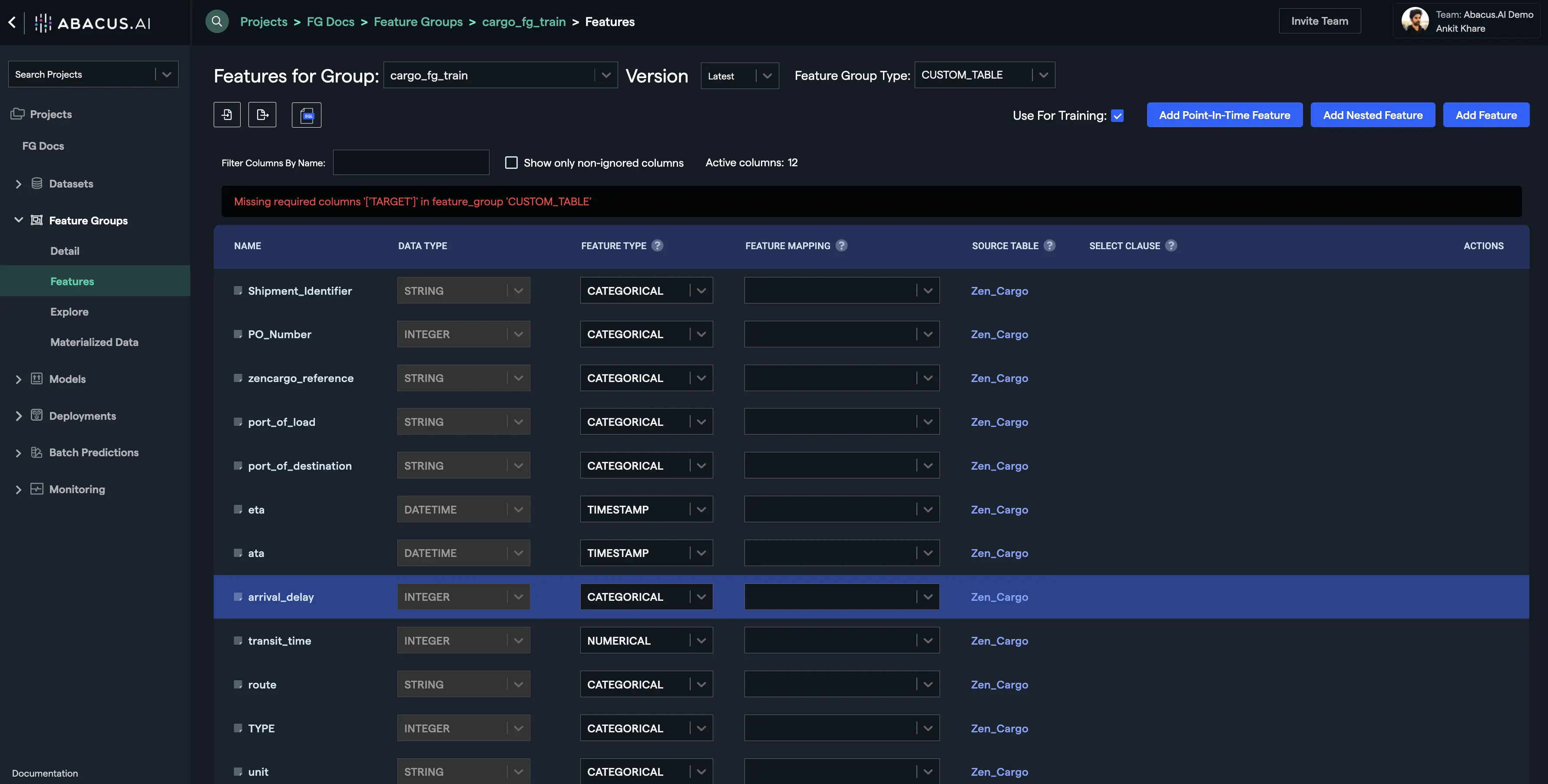
In the running example, let's say you need to predict the ratio of arrival_delay / transit_time. This can be done by adding a new feature under the "cargo_fg_train" feature group. On the left menu, select "Features" option under "Feature Groups". Now click on "Add Feature" button:
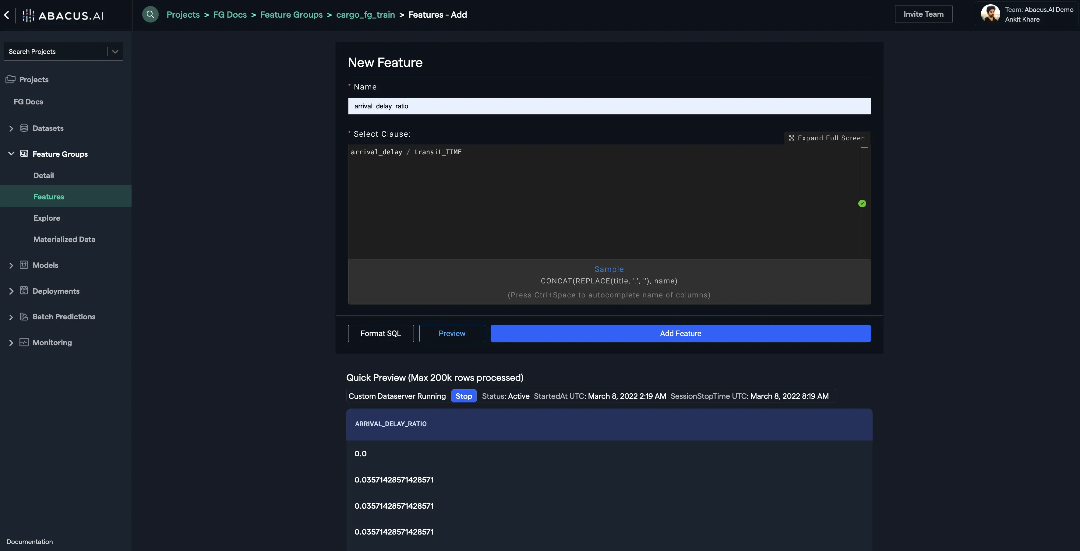
- Provide a name to the feature and write the "Select Clause" expression as shown below. You could also preview the output before adding the feature. Click on the "Add Feature" button to save your feature:
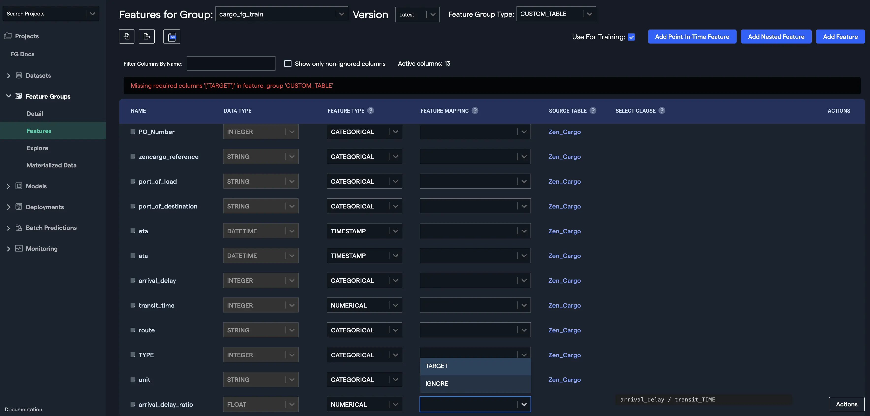
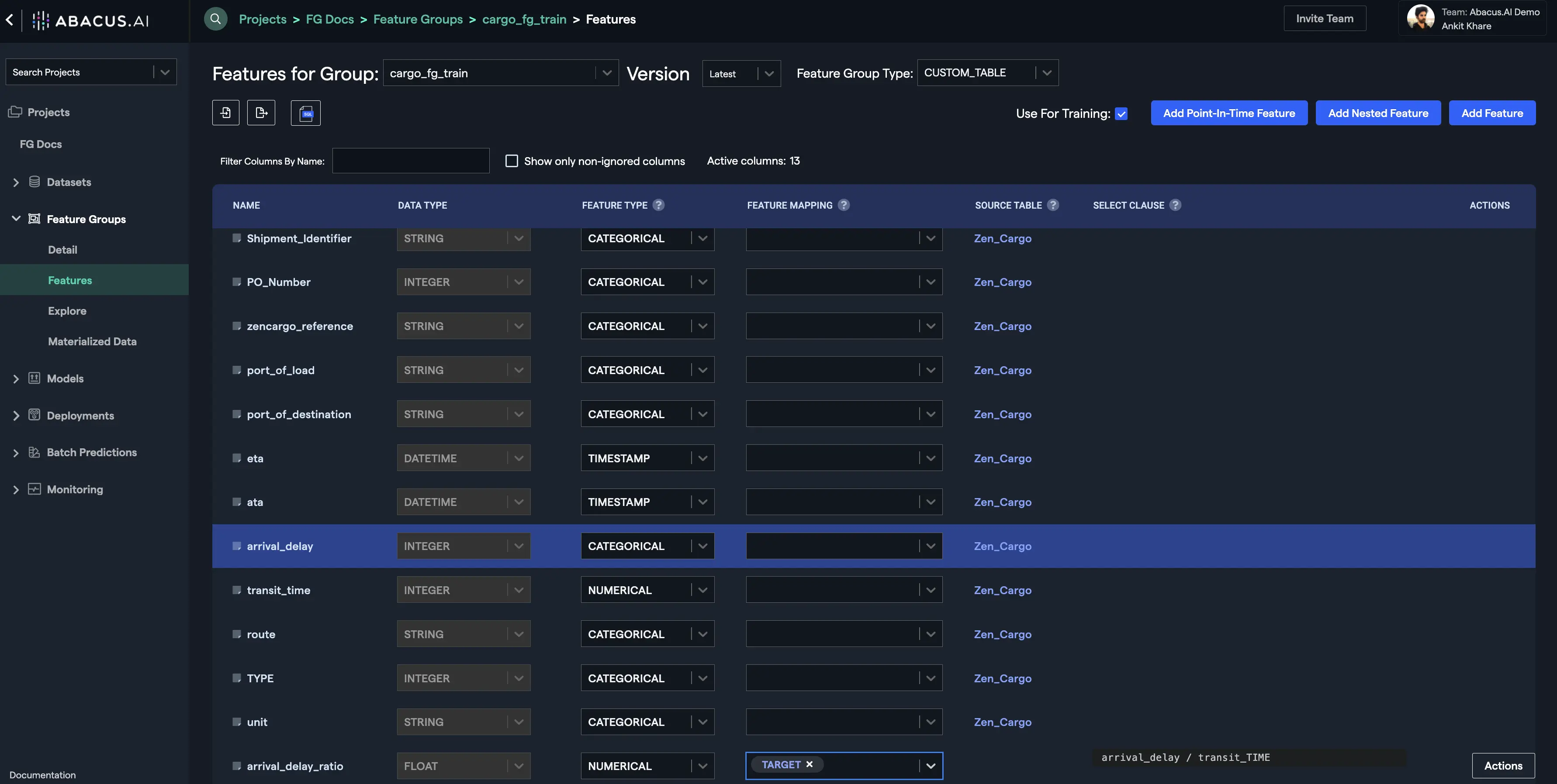
- Your new feature will be displayed at the bottom of the features list. You can provide a feature mapping to your new feature if required. In this example, the "TARGET" feature mapping is selected for the newly created feature and this also resolves the missing required columns error:
Point-In-Time Features
Overview
Point in Time features can be viewed as features created by applying functions such as the SQL window functions. PIT features are formed through calculations across a set of table rows. Point in Time features uses SQL-like aggregate functions such as MAX, MIN, AVG, etc., aggregate functions but operations are performed across a set of rows to get an output for the row and and every row maintains its state.
Example Steps to Create Point-In-Time Features
Let's see an example to understand how a useful Point in Time feature can be created and used later for training an AI/ML model:
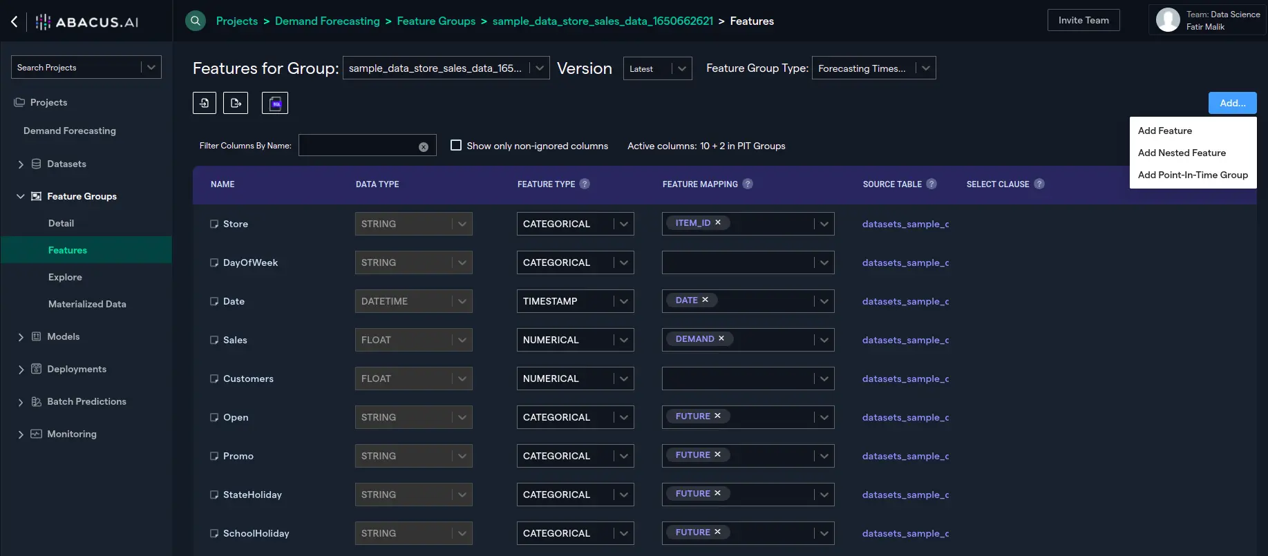
- Let's use a new demand forecast focused on store sales data. On the Feature Groups section select the Features option. click on the 'Add' button and select 'Add Point-In-Time Group':
- The following configuration window will be opened:
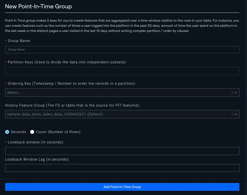
-
Let's say that we are interested in knowing the number of customers visiting a particular store in the last 10 days. We can create a Point-In-Time Group feature for this purpose by firstly naming our group and then setting 'Store' as our partition key because we are interested in knowing the customer count for each store. Then we need to set the Ordering Key which is mostly a Date or Timestamp.
-
For History Feature Group, the one attached to the project is selected as Default and we'll use it however we can choose any other feature group in the organization. Finally, we have to select the length of our feature that can be either a window of time or count. In our case, we're interested in the 10 last days so it's going to be a 864000 seconds lookback. If we were interested in last 10 sales for the store, we could have used last 10 rows as lookback. A "lookback window lag" defines how many previous timesteps in seconds or the number of rows are used in the subsequent "lookback window". It's '0' in our case as we aren't interested in adding a lag.
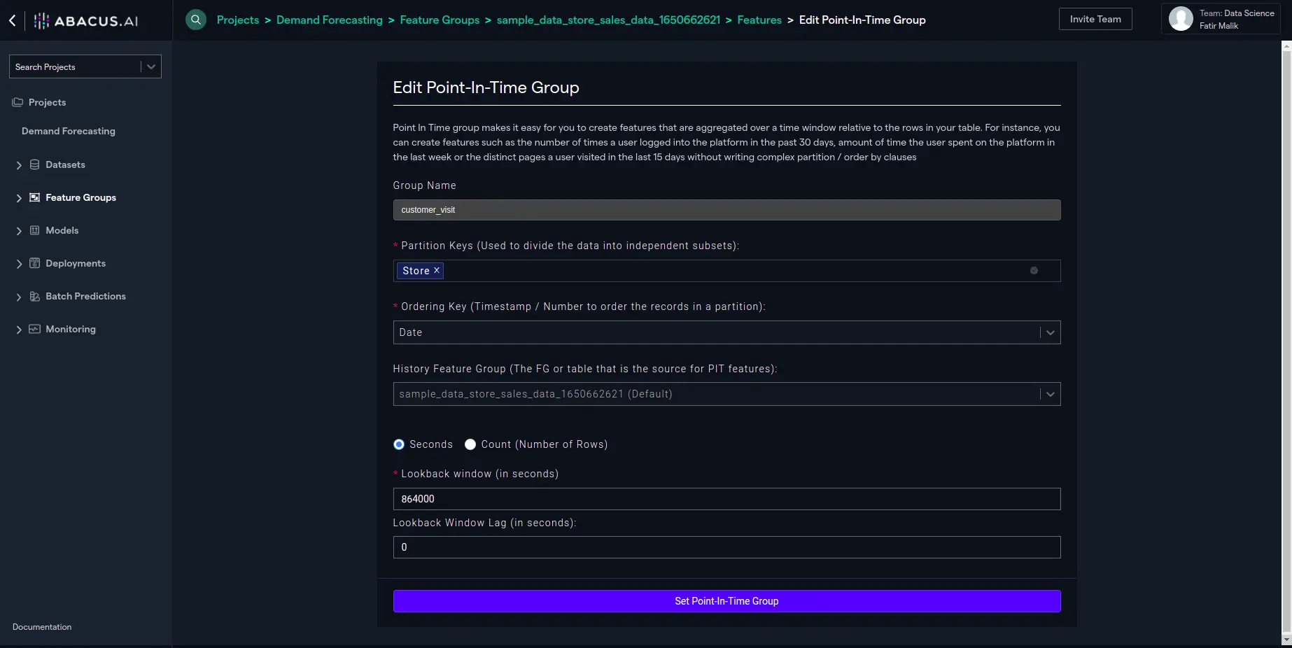
- Click "Set Point in time group" to set the PIT feature configuration:
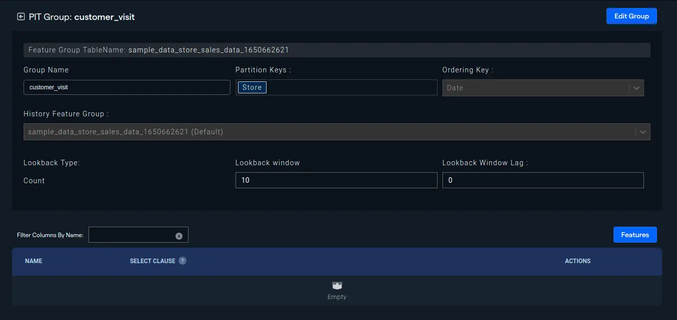
- Next, we will need to add the aggregate expression, i.e. SUM(Customers) in our case, to create the PIT feature:

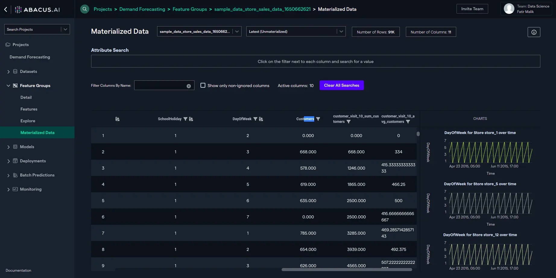
- To view the feature, we can go to the 'Materialized Data' and verify the intended behavior. The right-most column, 'customer_visit_10_sum_customers', shows the sum of customers visiting the store in the last 10 days:

- You can create multiple PIT features ,or instance, to find an average count of customers visiting the store in last 10 days, all you have to do from here is to add another expression, "avg(Customers)":

- Again, you can view the data using "Materialized Data" interface and see the newly created PIT feature:
Nested features
Overview
Real-world Machine Learning applied at enterprise data involves complex feature engineering steps. Flat tables are seldom sufficient to represent all the information needed to produce insights or predictions. Although, flat tables are good at capturing the static features within the training data, certain dynamic features are difficult to represent with flat tables. For instance, if you are trying to predict the probability of a user to churn, the flat table can represent the static attributes of the user such as age, geography, device, etc., however, dynamic features such as browsing activity, payment history, etc., cannot be captured easily using flat tables. Although you can manually engineer features for flat tables, but it is time consuming, error prone, and often does not allow ML algorithms to capture maximum information. This is where Abacus.AI's Nested Features comes into play. At the training stage, our AutoML and deep learning models are designed to extract maximum information from Feature Groups and Nested Feature Groups.
Steps to Add Nested Features
-
Let's say that you have two datasets, "user_info" and "interaction_data". The dataset "user_info" has several static features such as age, city, memberid, etc., and the dataset "user_interaction_data" has features like memberid, itemid, item_kept, category, etc. When you upload/attach these two datasets to your project, corresponding feature groups will be created for them with their respective table names as entered by you. Now, to take advantage of the user data as well as all the interaction data that the user has with the items in the catalog, you would nest the user_info feature group with an additional feature such that the "interaction_data" feature group will be encapsulated within your new feature. This is performed with the help of a simple "Using Clause". You can also specify a "Where Clause" and an "Order by Clause" for the join. Thus, interaction_data will be treated as Nested Feature Group for the user_info feature group.
-
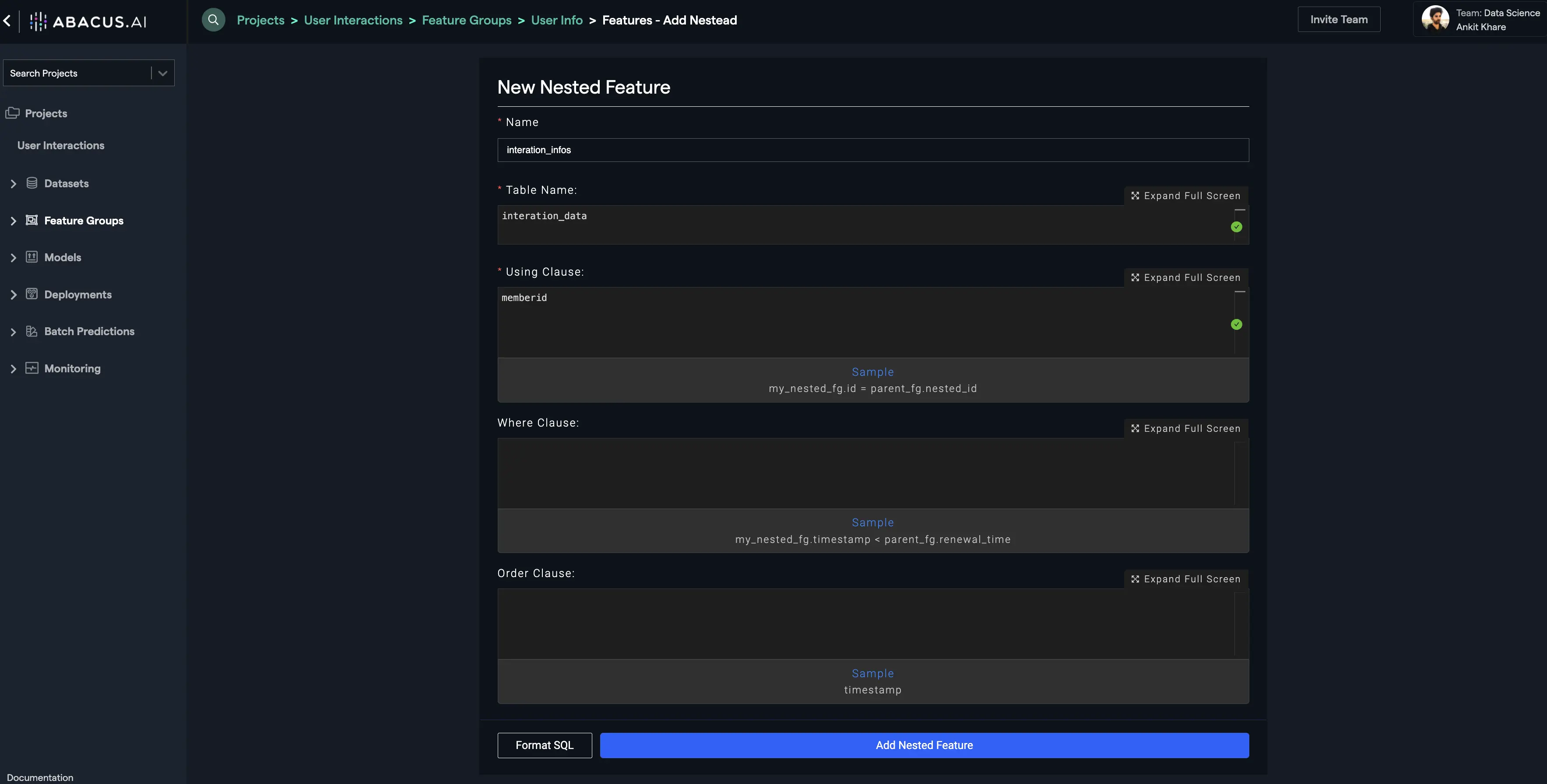
The first step is to click on the "Feature Groups" tab at the left navigation and select the "Features" sub-tab. Make sure that you have selected the user_info feature group at the top. Next, Click on the "Add Nested Feature" button. Enter the name of the feature group, the table to be referenced for creating the nested feature group (interaction_data for the current example), and the column/feature to be used under "Using Clause" as shown below:
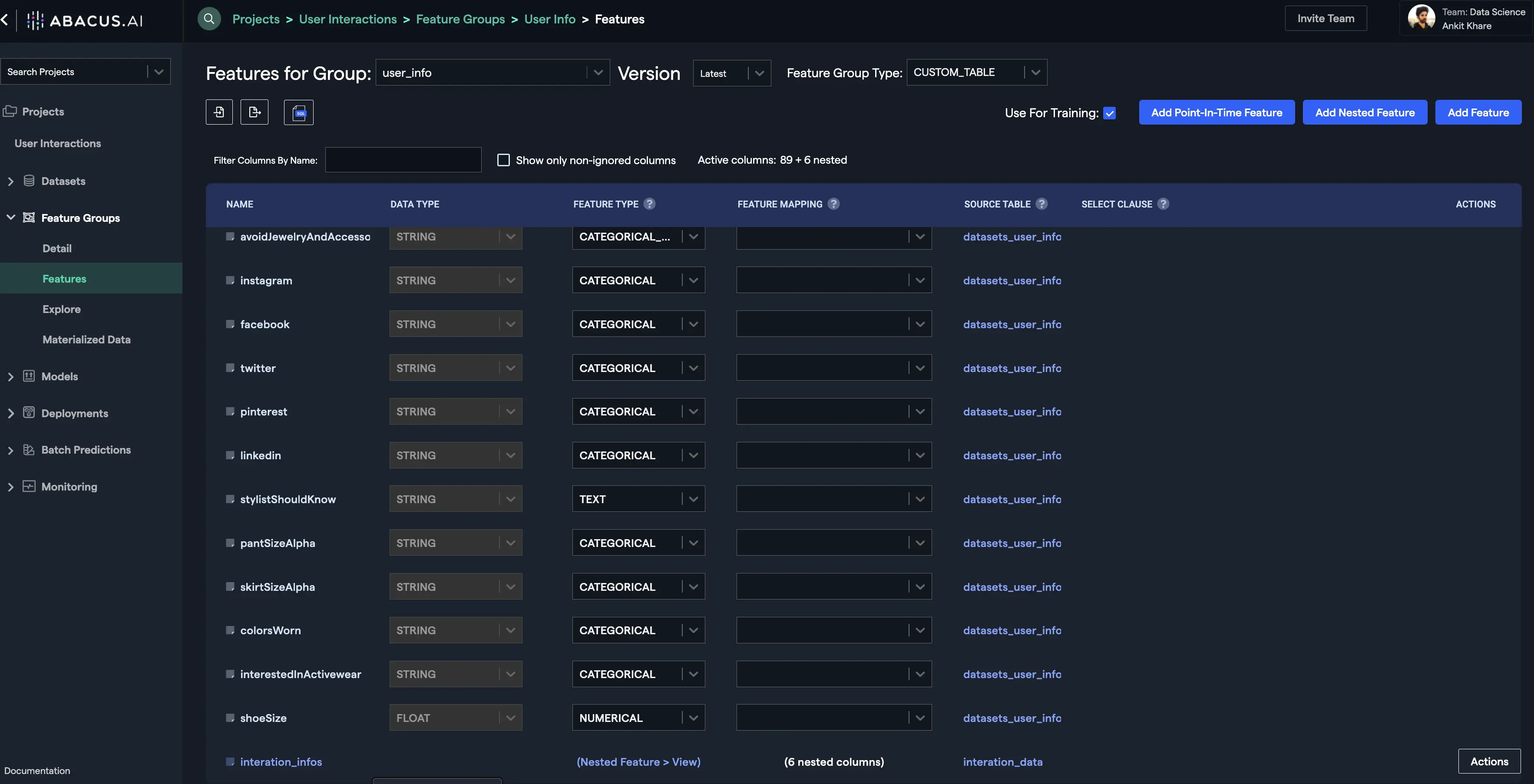
- Click on the "Add Nested Feature" button. You will find your nested feature as the bottom-most feature:
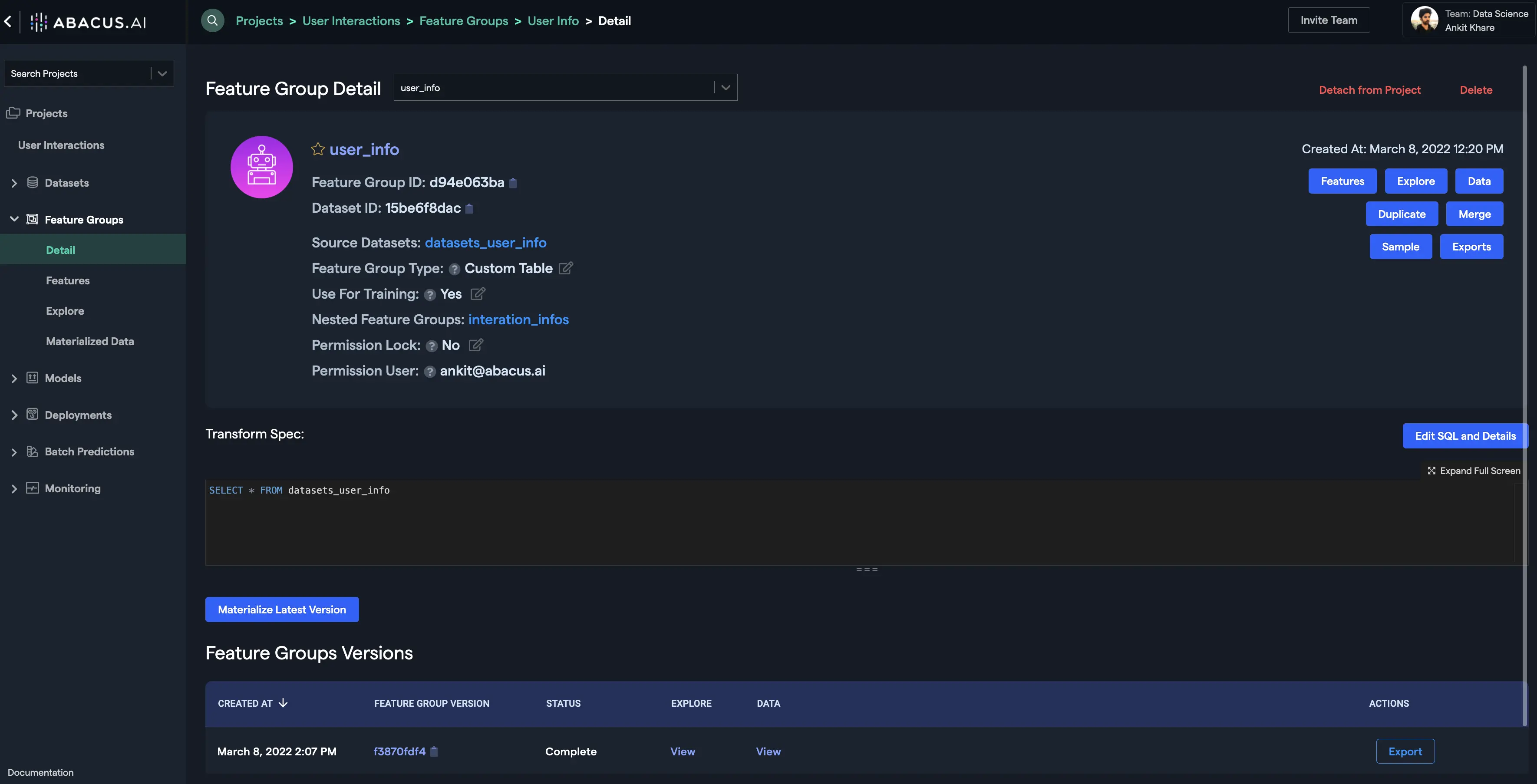
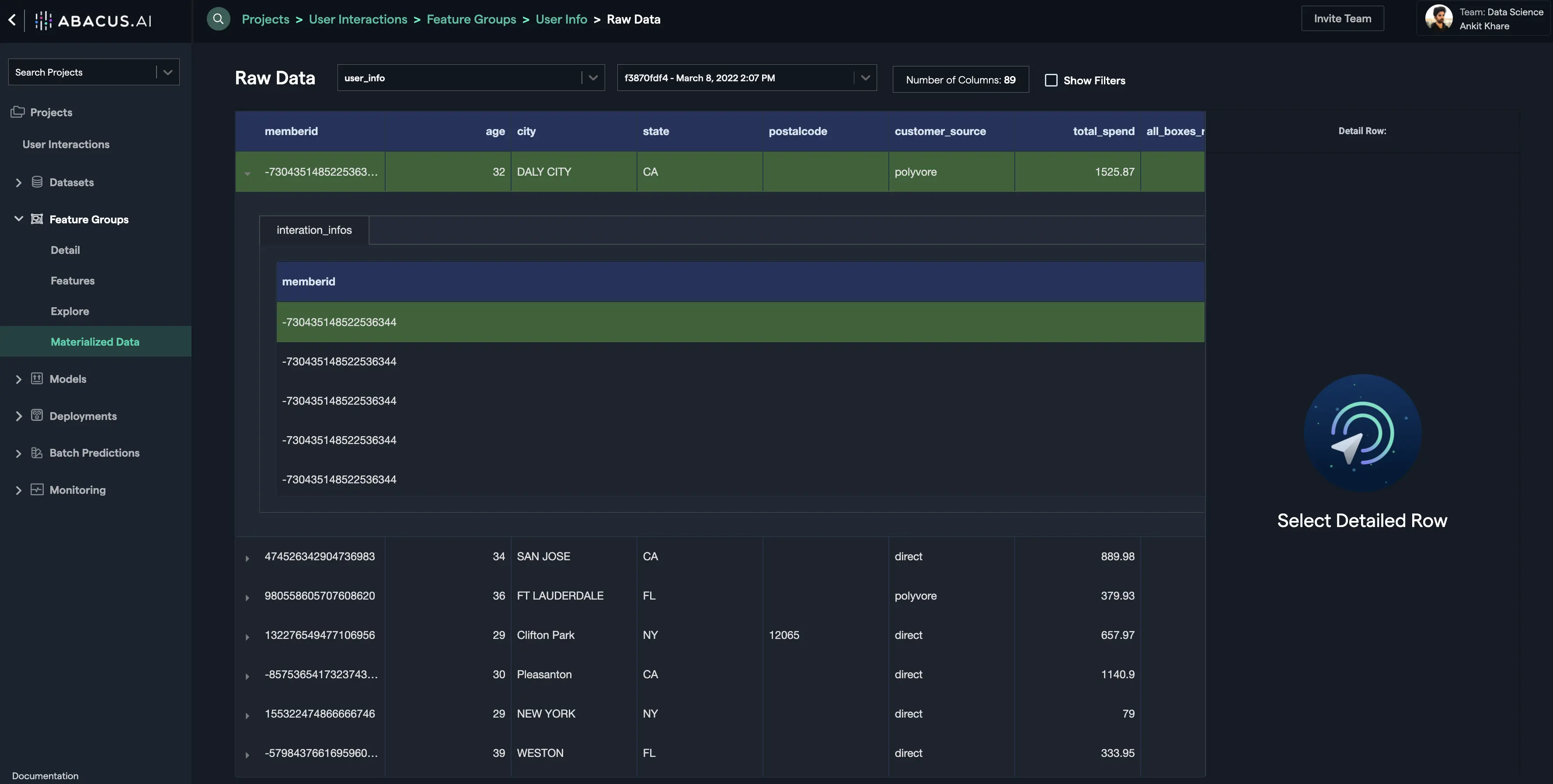
- You can visualize the data within this feature group by materializing the feature group. Click on the "Materialize Latest Version" button and wait for the process to finish. Once it finishes, click on the "View" button under the "Data" column of the feature group version to visualize the data:
- Notice the downward pointing arrow on the rows. Click on any of them to see the nested feature group data for that row:
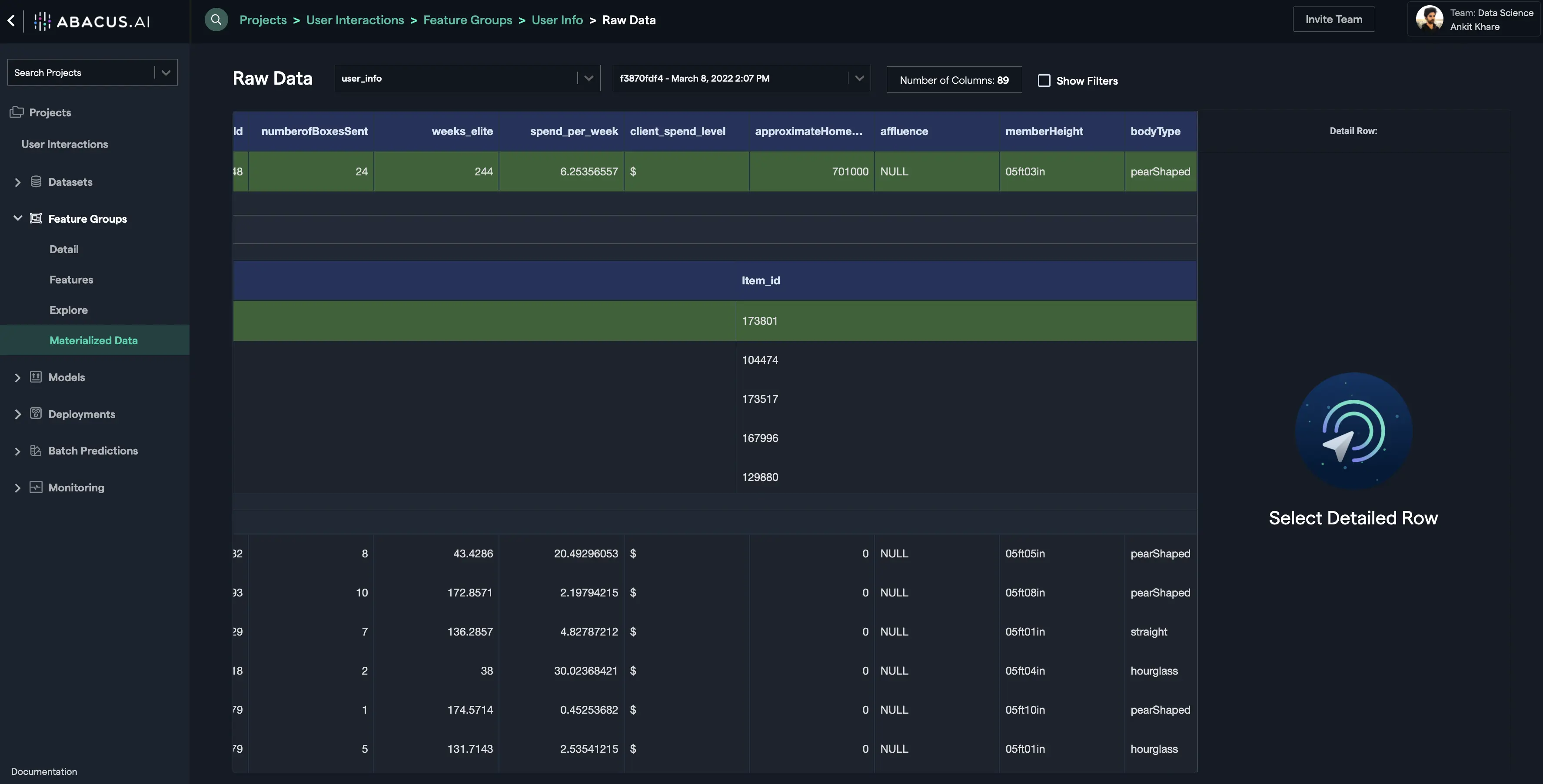
- Scroll right to see other columns:
This is how the nested feature group helps make it effective and efficient to represent the dynamic nature of the ML features and makes it possible for the ML algorithms to get the most out of the complex real-world data.